The goal of this two-part blog series is to identify areas of extreme slope, and then class based on aspect. We covered the first part in part-1, linked here.
In part-1 we discussed some of the applications of slope and aspect analysis including natural hazard assessments, urban planning and more. Identifying extreme slopes is intuitive. Cliffs, and steep hills pose a challenge or threat to people, communities and the environment. But the aspect plays an important role too. A moderate slope in the mountains may pose an extreme avalanche risk due to the compounding effect caused by its aspect exposing it to more afternoon sun which may soften the snow. Whereas the same slope on another aspect may not pose the same risk. Or in biodiversity conservation, a cliff dwelling fern may be more prevalent on aspects that point away from the sun to stay cooler.
In the previous blog post, we created a slope map that showed locations of the Grampians in Victoria that were greater than 30%. We did this mostly through symbology by creating the slope map, and turning all areas that were less than 30% transparent, and all areas greater than 30% red. Now we will add aspect to the equation too.
Multiple pathways, same result
The obvious choice is the aspect-slope raster function.
Surface raster functions in ArcGIS Pro
This creates a view of your data symbolized by aspect and slope that you can further customize. If hitting that button gives you everything you need, then perfect. Lets call it there, and good luck on your journey. This beautiful result is what you’ll see.
Aspect Slope raster function.
There are also ways of masking the data using the previously created data, but today we’re going to get a bit deeper by reclassifying and creating a new layer. Why? Because this is an instructional tutorial so we’re going to take the scenic route.
Just aspect
To reinforce the previous exercise, we’ll perform the same workflow as part-1, but with the aspect raster function.
Open the Aspect raster function, point it at your Terrain DEM and click run.
An aspect raster created from ArcGIS Pro.
Then we will symbolize based on cardinal direction. Where north is 0 degrees, east is 90, etc. So we need to find the halfway point of each of these.
Symbolizing aspect by cardinal direction.
In this example, we left the colour ramp as a graduated colour ramp, but it would be much more useful to make the colours disparate so the different aspects can be more clearly identified.
Aspect map.
So there you have it. The aspect map. You can make whatever modification you like such as showing only a certain aspect (by making all others transparent), or any other variation. Next we will hard code it using the reclassify tool.
Reclassify
Why reclassify? There are a number of reasons including:
More control and customisation
Output as permanent raster
Enhanced analysis capabilities
Performance with large datasets (as oppossed to processing on-the-fly)
Error reduction by using “missing values” and “Assign NoData” options
Data integrity in complex workflows.
So lets do it:
Reclassification tool to display aspect
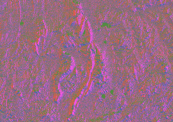
This is similar to the symbology settings we setup earlier. The output is verging on data art …
Aspect map created by the reclassify tool.
Repeat this, but for slope. That is, reclassify areas with slope that is greater than 30% as 1, and all others as 0.
Combining aspect with slope
There are a number of ways of doing this next part. You can create a multidimensional raster, or use the raster calculator to add them together. The latter is probably what I would do if I were to leave it in raster format. for example, You could assign areas greater than 30% a value of something high, like 1000, and all other values 0. Then add the two rasters together. Something with a northerly aspect of 350 degrees on a moderate slope will retain a value of 350 in the raster. However, something on a steep slope (>30%) will have a value of 1350 in the raster. Therefore you can ignore the values less than 1000 to display on steep areas.
However, just to slip another workflow in, we’re going to convert to polygon and work with vector data.
Both the aspect and slope layers need to be polygonized.
The raster to polygon tool in ArcGIS Pro.
And then it is as simple as clipping on to the other and symbolizing.
Clipping aspect from slope.
And there you have it, our final map showing areas where the slope is greater than 30%, classified by cardinal direction.
Steep slope and aspect symbolized by cardinal direction.
As mentioned, there are a bunch of different ways to achieve the same result. We just took the scenic route to show a few different workflows in ArcGIS Pro.


